Dec 11, 2022 6 min read sql-patterns

How to Write Modular SQL

In this post we're going to learn one of the most important patterns in SQL: Modularity.

In this post we're going to see how modularity, one of the most important system design principles applies to SQL.

Definition:
A module is a unit whose elements are tightly connected to themselves but weakly connected to other units.

When a system is designed with modularity in mind, it makes it very easy for independent parties to build these components in parallel so they can be assembled later. It also makes it easy to debug and fix the system when it's in production.

Modularity is one of the core principles of the design of operating systems. If you're familiar with the command line interface on a Mac, you've seen its power. It's designed in a way to stitch together independent tools to solve ever more complex problems.

In this post we'll learn how we can apply it to SQL.

Three Levels of Modularity

In SQL we can apply modularity in 3 different levels:

Within the same SQL query
Across multiple SQL queries
Beyond SQL queries

Have you ever written or debugged a really long SQL query? Did you get lost in trying to figure out what it was doing or was it really easy to follow?

Whether you got lost or not depends a lot on whether the query was using CTEs to decompose a problem into logical modules that made solving it and understanding it really easy.

Level 1 - Within the same SQL query

CTEs or Common Table Expressions are temporary views whose scope is limited to the current query. They are not stored in the database; they only exist while the query is running and are only accessible in that query. They act like subqueries but are easier to understand and use.

CTEs allow you to break down complex queries into simpler, smaller self-contained modules. By connecting them together we can solve any complex query.

Side Note:
Even though CTEs have been part of the definition of the SQL standard since 1999, it has taken many years for database vendors to implement them. Some versions of older databases (like MySQL before 8.0, PostgreSQL before 8.4, SQL Server before 2005) do not have support for CTEs. All the modern cloud warehouse vendors support them.

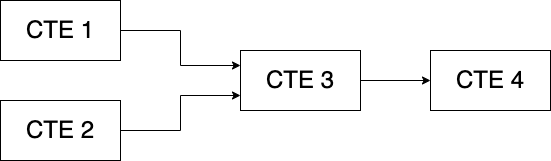
One of the best ways to visualize CTEs is through a DAG (directed a-cyclical graph). Here are some examples of how CTEs could be chained to solve a complex query.

Here's the first diagram and its corresponding code.

In this example each CTE uses the results of the previous CTE to build upon its result set and take it further.

-- Define CTE 1
WITH cte1_name AS (
    SELECT col1
    FROM table1_name
),
-- Define CTE 2 by referring to CTE 1
cte2_name AS (
    SELECT col1
    FROM cte1_name
),
-- Define CTE 3 by referring to CTE 2
cte3_name AS (
    SELECT col1
    FROM cte2_name
),
-- Define CTE 4 by referring to CTE 3
cte4_name AS (
    SELECT col1
    FROM cte3_name
)
-- Main query
SELECT *
FROM cte4_name

Here's another diagram and the corresponding code.

In this example, CTE 3 depends on CTE 1 and CTE 2 which are independent of each other and CTE 4 depends on CTE 3.

-- Define CTE 1
WITH cte1_name AS (
    SELECT col1
    FROM table1_name
),
-- Define CTE 2
cte2_name AS (
    SELECT col1
    FROM table2_name
),
-- Define CTE 3 by referring to CTE 1 and 2
cte3_name AS (
    SELECT *
    FROM cte1_name AS cte1
    JOIN cte2_name AS cte2 
        ON cte1.col1 = cte2.col1
),
-- Define CTE 4 by referring to CTE 3
cte4_name AS (
    SELECT col1
    FROM cte3_name
)
-- Main query
SELECT *
FROM cte4_name

Finally here's something more complex and its corresponding code.

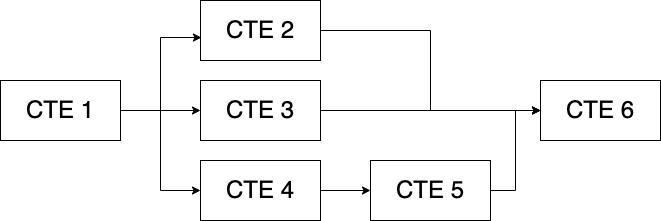
As you can see, there's an endless way in which you can chain or stack CTEs to solve complex queries.

-- Define CTE 1
WITH cte1_name AS (
    SELECT col1
    FROM table1_name
),
-- Define CTE 2 by referring to CTE 1
cte2_name AS (
    SELECT col1
    FROM cte1_name
),
-- Define CTE 3 by referring to CTE 1
cte3_name AS (
    SELECT col1
    FROM cte1_name
)
-- Define CTE 4 by referring to CTE 1
cte4_name AS (
    SELECT col1
    FROM cte1_name
),
-- Define CTE 5 by referring to CTE 4
cte5_name AS (
    SELECT col1
    FROM cte4_name
),
-- Define CTE 6 by referring to CTEs 2, 3 and 5
cte6_name AS (
    SELECT *
    FROM cte2_name cte2
        JOIN cte3_name cte3 ON cte2.column1 = cte3.column1
        JOIN cte5_name cte5 ON cte3.column1 = cte5.column1
)
-- Main query
SELECT *
FROM cte6_name

Level 2- Across multiple queries

When you find yourself copying and pasting CTEs across multiple queries it's time to refactor them into views, UDFs or stored procedures.

Views are great for encapsulating business logic that applies to many queries. They're also used in security applications to limit the rows or columns exposed to the end user based on their permissions.

Views

Creating a view is easy:

CREATE OR REPLACE VIEW <view_name> AS
	SELECT col1
	FROM table1
	WHERE col1 > x;

Once created you can run:

SELECT *
FROM <view_name>

This view is now stored in the database but it doesn't take up any space (unless it's materialized) It only stores the query which is executed each time you select from the view or join the view in a query.

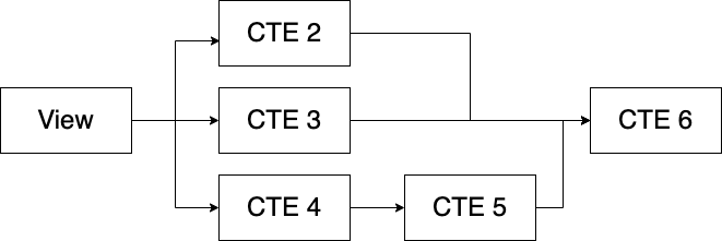
Views can be put inside of CTEs or can themselves contain CTEs, thus creating multiple layers of modularity. Here's an example of what that would look like.

Side Note:
By combining views and CTEs, you're nesting many queries within others. Not only does this negatively impact performance but some databases have limits to how many levels of nesting you can have.

UDFs

Similar to views you can also put commonly used logic into UDFs (user-defined functions) Pretty much all databases allow you to create UDFs but they each use different programming languages to do so.

SQL Server uses T-SQL to create functions. PostgreSQL uses PL/pgsql or Python (with the right extension) BigQuery and Snowflake use Javascript, Python, etc.

Functions allow for conditional flow of logic and variables which makes it easy to implement complex logic.

UDFs can return a single scalar value or a table. A single scalar value can be used for example to parse certain strings via regular expressions.

Table valued functions return a table instead of a single value. They behave exactly like views but the main difference is that they can take input parameters and return different tables based on that. Very useful.

Stored Procedures

Like table-valued functions, stored procedures (sprocs) allow you to encapsulate very complex business logic inside a database. They also return tables as their output.

They were heavily used in transactional systems to implement business logic inside the database, but have fallen out of favor in data processing. I will not cover them here.

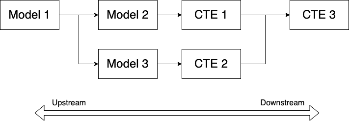
Level 3 - Beyond SQL Queries

With the advent of tools like dbt (Data Build Tool) you can move beyond views and CTEs for your queries to build more complex dags that combine all of them.

In dbt lingo, views and tables are known as models. By using the function ref() dbt enables referencing previously built models. You can also mix and match CTEs with models to achieve the desired result.

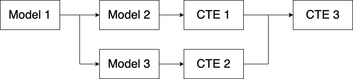
Here is how this looks in practice:

model_a.sql

select *
from public.raw_data

model_b.sql

select *
from {{ref('model_a')}}

How to decompose a query into simpler modules

Now that you've seen the theory behind query composition, how do you apply it? As you're writing a query, you apply one of the following 3 rules. They apply equally to all 3 levels.

Rule 1: Don't Repeat Yourself (aka the DRY principle)

The DRY principle states that if you find yourself copy-pasting the same chunk of code multiple times in the query, you should put that code in a CTE and reference that CTE where it's needed.By putting repeated logic into separate modules, you make it easy on yourself to write, maintain and debug code.

Rule 2: Make modules single-purpose (aka the SRP principle)

The single responsibility principle (SRP) in software engineering says that every module should be self-contained and only have a single purpose. The module could be a CTE, a view or dbt model.

By being self-contained and having a single responsibility, each model can be written, tested and debugged independently. Dbt increases your flexibility multiple times by allowing you to create macros or functions (UDFs) to offload responsibility to.

Rule 3: Move logic upstream

When you find yourself implementing very specific logic in a model that might be used elsewhere, move that logic upstream as soon as possible.

In the world of DAGs, upstream has a very precise meaning. It means to move potentially common logic onto earlier nodes in the graph because you never know which downstream models might use it.